Bringing it all home and making it special....

So, we continue our "Back to Basics" blog run this week. I want to look at the "taken for granted and normally ignored" Home menu.

Yes, this menu contains so many tools that you probably use all the time, you would be forgiven for not investigating any of the more obscure icons. That is what I am for....
 
First off I want to go over some of my favourite tools for making your spreadsheets look good (and it's all about looking good, don't you know! ) I have gone over these in detail in a number of my previous blogs, but for a quick recap:
 
Format Painter
 

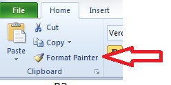This is a fabulous little brush. Use it to copy the formatting from one cell to other cells. So if you had a group of cells that were formatted exactly as you wanted them, and you wanted to copy that formatting to another group of cells, all you do is highlight the formatted cells, click on the format painter, and then click on the cells you want to format. That's it.

 

 

Styles

 



The Styles Menu lets you easily format your cells to pre-designed formats. You can select from the options available by simply clicking on your preferred style type while you have your cell highlighted. You can also adjust the styles available, so for example make the text in the block "Accent 4" bold and italic, by right clicking on the "Accent 4" block and selecting "Modify".
 
These styles will apply to all your worksheets within a workbook. A nice way to ensure all your sheets look uniform and smart.
 
And now for something completely random....
 
I find this next tool really useful for highlighting specific cells. So, for example, you have filtered a number of rows, and you want to delete the data in your filtered cells, but leave the "hidden" rows untouched. You could delete each cell's data separately. You could trust in the goodness of Excel that if you just highlight all the cells and press delete it won't delete the underlying cells. (Sadly, this has happened to me once too often, and the trust has gone, so I am always extra cautious).
 
Or,  you could just use the "Go To Special" tool, which you find here, right at the end of the home menu...
 

 
 
Click on this, and you get a table of various options you can select. For our example, you would use "Visible Cells only".
 
 
 

 

If you just wanted to select all the blank cells in a selection, you select (funnily enough) "Blanks" and so it goes on....

This is just a handy little tool for finding specific types of cells, and one that I have discovered not so  many people are aware of.

So those are my random helpful icons for today. Again, if you have any questions, please feel free to add a comment or get in touch with this link.

Thanks for reading, and happy spreadsheeting!
 
 

Back to Basics - Do you know your icons?

Hi and welcome back.

I know I have been a bit quiet on the blog front recently, but that is just because all my other fronts were demanding my attention! But I missed keeping in touch, so I am back with a new series of Excel blogs. They are going to follow my father's rule of keeping everything "Short, sweet and to the point".

So these missives will be shorter than my previous posts, but will hopefully still be as useful. And they will be all about getting back to basics. Knowing all you can about the easy stuff in Excel so you can practise it, make it perfect, then not even think about it while you use the easy stuff to do the hard stuff.
 
As always, if there is any little (or big) issue in Excel you would like me to address, please feel free to leave a comment or send an email through this link.

In the first few blogs in the "Back to Basics" series, we are going to get to know the menu ribbon. I will randomly select different icons off the ribbon and tell you what they do. You should hopefully learn something interesting each time.

Our first icon looks very unassuming and innocent but is probably one of the most powerful icons on the ribbon. It's this one:

Yup - that tiny little arrow you may have thought was just window dressing,  actually allows you to add any tool you want to your Quick Access Toolbar, which is the top line of icons above the menu bar. Why this is handy is that you can add any tools you use frequently to the Quick Access Toolbar, and then you don't need to scroll though your menus to find them.
 
You can also add tools that aren't necessarily available on your menu. By clicking on the icon circled above, you can select the option More Commands... and you will get this:

Choose the type of commands you want to look through from the dropdown selection at the top left hand side, click on your selected tool icon on the left, click Add, Ok, and you're done.

You might notice this little icon I have added to my own Quick Access Toolbar:
 

 
This little gem is a wonderful time saver. Click on this, and it will open a list of your recent workbooks and places, making finding files you have been working on a lot easier. It also allows you to "pin" a workbook so that workbook always appears at the top of your list. Even if you haven't opened it in months. Just click on the little picture of the thumbtack to the right of the workbook name, and you're sorted.

How to add it is simple. Once your have your "Customize your Quick Access Toolbar" Menu open, select All Commands from the drop down list, and then go to the command "Open Recent Files" (the commands are listed alphabetically), and add it.
 
So, there you go. Short and sweet, and 2 little handy tips to brighten your day!
 
Have a great one!

Don't waste time on "what if's"....

Have you ever sat in your cosy little office, or claustrophobic little cubicle, and daydreamed? I'm certain you have, and no doubt it was about your holiday, your children, your boss being challenged to a duel at dawn....but have you ever dreamt of finding a way to cut down on your mundane, boredom inducing, life wasting Excel tasks? Like data entry?

Well, daydream no more, because here is a quick and easy little tip that might just make your workload that tiny bit lighter, leaving more time for daydreaming of important things. What's that? You would naturally spend that time doing more value added tasks?....ofcourse you would!!

Anyway, the reader's question was, "When inputting invoice data into a spreadsheet, and each invoice contains a number of items, is there a way I can set up my spreadsheet so that I don't have to re-enter the invoice number and date for each line item?"

There is, and this can be used for any type of data entry that requires repetition of certain cells within a group of lines.

So imagine your data spreadsheet looks like this:

If you are going to add different lines to the same invoice number 1012, then simply use the following formulas in columns A and B (I have them in different colours to make it easy to read here):

You can drag these formulas down for as many rows as you like. They will remain blank until you add in detail into column C. To make sense of the formula, you need to read each formula as saying, "If cell C5 (or whatever line you're on) is empty, then make this cell blank, otherwise copy the data from the cell above."

So if you now add detail into cell C6, the date and invoice will immediately be copied from above. Obviously, a major point to remember is to change your invoice numbers and dates for each new invoice. You can simply type over the formulas in the next line down, and start entering your product details.

Easy as pie and a time saver of note if you have to add a huge number of invoices.

To take this one step further, and make this type of invoice entry even quicker, I would create a standing table of product data, which has all your product details per product code. So it may look something like this:

If you saved it into the same workbook, it would save space. I would then create a dropdown list in your invoice entry sheet in column C, to look up the product codes. To do this, you would use Data Validation (click here for my prior blog for guidelines). You could then use VLOOKUPs to bring back all the relevant information for each product code. (read here for a comprehensive guide to VLOOKUPs).

Using all these tools, you could set up your worksheet so that you only enter your invoice number and date once, you select each product code as required, and enter the quantity. Everything else will fall into place automatically. You could almost go on that holiday, not just daydream about it.

One IMPORTANT point....if you update your product data table with price changes etc, first copy and paste value all the invoice lines you have already entered, otherwise all the previous invoice lines will pick up your new changes!

If you would like to get a friendly reminder of each new blog post, please sign up here.

Happy Halloween, and hope your spreadsheets don't break out in gremlins!

Did you hear that one about the accountant...?

Why is it that poor old accountants are the butt of so many bad jokes? They get so much flack for doing such a thankless task. My personal favourite accountant joke....What does an accountant use for contraception? His personality.

Now, now, before I get loads of complaints, I'm an accountant too...and if we can't laugh at ourselves, 'tis a sad life. And why I am bringing out the  bad accountant jokes? Because I am about to head into serious accounting territory, so wanted to get you all loosened up first!

Ok, this is not as serious as having to re-do your tax returns, but I have been asked a specific accounting type question, so will answer it with an accounting based solution. However, please note that while I have recreated a P&L and Trial Balance, you will note that they are a "little" basic and only cover sales and cost of sales. This is because it still conveys the answer required, and doesn't take up heaps of space.

So, the question I was asked was....how do you create a rolling P&L, with each months' figures next to each other, without having to manually key in the figures from separate spreadsheets? I'll show you my solution, and there lots of ways of doing this, but this is the one I like for simplicity:

Lets assume you download a Trial Balance each month and save it somewhere. Lets also assume that your Trial Balance is governed by account numbers. So it looks something like this:

(Before all the accountants start yelling that a Trial Balance should net to zero, like I said, this is fictional and incomplete!)

You also want to have a P&L that looks something like this:

Please note the column headings - they jump from D to O because I have hidden the other columns, which contain March to December, until needed.

So, instead of having to type in each month's figures, or set up a fresh lookup formula and copy it all the way down, you can set this all up using an INDIRECT formula embedded in a VLOOKUP. I briefly touched on this in a prior blog, but I will take you through it step by step now.

First thing is in the set up. Obviously you want to set up your P&L to look just right the first time round. So do it, but only do all the formulas etc for the first month. Once you have it perfected, drag all the formulas across the rest of the columns.

Second thing is, it is better if you paste each month's trial balance into a new sheet within the workbook. This is because an INDIRECT formula will bring back an #REF! error if the workbook it is looking up to is closed.

Right, I have pasted my Trial Balances into my workbook for January and February, and my tabs look like so:

To keep this as simple as possible, I have just shown one formula (for Sales for Widget A) and some of the other more basic formulae:

Now, the step by step walk through (its not nearly as scary as it looks):

IFERROR - this formula is saying "if the results of the following formula comeback as an error, then return 0 instead". That is what the 0 at the end of each line is for. This will also make sure your YTD total doesn't show errors when you drag the formula across for future months.

VLOOKUP - this is your basic VLOOKUP formula as discussed in prior blogs (click here for a refresher). The first brings back your Debit totals, and the second brings back your Credit totals, and these are added together for a total for each account number. This example is based on account numbers, but you can use anything as long as each line is unique. So descriptions are fine too, just make sure the spelling is identical in both sheets.

INDIRECT - instead of  having to set up the formulas each month once you have your TB file, you simply point your lookup to the month name in row 3, and if your sheet is named the same, it will perform the lookup in that month's sheet. So when you add in your February figures to the sheet named Feb, it will automatically lookup the numbers. Just be sure to check the TB data is always in the same columns.

Once you have this setup, it really is as simple as pasting a TB into a sheet in your workbook to update your YTD P&L - obviously unhide each month as you need it.

One word of warning - it is always a good idea to have some kind of automatic sum check to compare your P&L totals to the sum of the P&L accounts in your TB. I haven't put a solution in here as everyone's TB will look different, but just bear it in mind. Sometimes automating things too much can make you miss some crucial points (or new TB accounts!).

If you would like a friendly reminder of all new blogposts, please sign up here.

Happy Spreadsheeting!

Now we're smokin'.....

So, last week's blog on branding your work seemed to hit a couple of spots...and a big thanks to all who have written in or commented. I am delighted that so many of you found this useful, and I am positively ecstatic that you wrote in with further questions on the subject matter.

(Side note - please feel free to email me or comment with questions or suggested topics for this blog...it makes me have to think less, which is always welcome!)

Right, lets get to it. Last week we looked at how to create a standard template which opens every time you open Excel. Why would you do this? To save time and create a fabulous, unique brand for your Excel output.

If I can summarise the emails/comments I received into 3 main questions:

1) Once you are already in Excel, how do you get Excel to give you your lovely, newly formatted workbook every time you press Ctrl N, instead of giving you the boring old default workbook?

2) How do you get your new formatting to apply to new sheets you add to your current workbook?

and

3) Can you have more than one specially formatted workbook?

The solutions to these points are very similar (use an Excel template), but have very specific differences in implementation, so take heed of the answers:

Question 1:
Once you have followed the steps in last week's blog, you will have succeeded in saving an Excel Workbook into your XLStart folder, which ensures you get your new template every time you start Excel.

If you want every new workbook you create to look like this, without having to re-open Excel, then save your Workbook into the same XLStart folder, BUT save it as an Excel Template (*.xltx), and VERY IMPORTANT - name it as book.xltx. Don't accept any names your helpful pc might suggest, as this will only work as book.xltx.

So, just to be sure to be sure (as us Irish would say):

a) Make sure it is in the XLStart folder (as soon as you select Excel Template, your PC might helpfully direct you to a Template folder...push the back button to get back to the XLStart folder)

b) Make sure it is named book.xltx (unless you have Macros in your workbook, then save it as an Excel Macro-Enabled Template (*.xltm))

Once you have done that, if you are in Excel and press Ctrl + N, your newly formatted Workbook will appear, as opposed to the standard default option.

If you are ever feeling nostalgic and want to get the standard Microsoft default workbook back, go to File - New - Blank Workbook.

Question 2:

To apply your formatting to new sheets you add to your workbook, you follow the same steps as above, with two small differences:

a) Make sure your formatted workbook contains only one sheet, and make sure that sheet is formatted as you want all new sheets to be, and

b) Save your sheet into the XLStart folder as an Excel Template BUT name it sheet.xltx.

Simple as... Now, when you're in Excel and add a new sheet, it should be formatted with your new brand!

Question 3:

What if you need to have a range of different templates? Handy if you prepare analysis for different companies with different colour schemes, for example.

To do this, create your first workbook in the design and layout you need. Now you are going to save this as a Template too, but you save it into the Template folder which Microsoft suggests. So click Save As, and select Excel Template (or Excel Macro-Enabled Template) from the dropdown list:

Make sure the Template folder comes up (as above) and save your Template with an appropriate name. You can repeat this for as many different templates as you need.

When you need to use a specific template, you just need to be in Excel. Go to File - New - My Templates:

The following little box will pop up with your selection of Templates:

Pick your template and you're sorted.

One word of warning - remember to save your newly opened workbook as something else immediately, or as soon as autosave kicks in, your template will be changed!

If you would like a friendly reminder to read this blog whenever there is a new post, please subscribe here.

Thanks for reading, and happy spreadsheeting!

Brand it like Beckham...

Brand Beckham. Known worldwide. He is handsome but rugged, a man's kind of man on the field, a woman's kind of man with children and fashion. She is forever pouty, perfectly groomed, and her fashion label is growing beyond anyone's expectations...besides maybe her own.
 
So how do they do it? I'm no marketing guru, but what strikes me most about the couple is that there is almost a uniform look about them. Their looks never change too drastically, they have a style and they stick to it. Victoria's fashion lines are instantly identifiable as hers with their clean cut lines and simple, yet always smart, designs. I mean, who doesn't immediately recognise these two?
 

 
 
So well done them...branding done right. But do you know that you can brand your own Excel work? You can, I've done it. Most of my colleagues could open one of my workbooks and instantly say, "Oh Vicky, this is one of yours, isn't it?" How did I do it? I certainly didn't have "Vicky's workbook" emblazoned across the top. I try be a bit more subtle than that....
 
You may have noticed through my blogs that I like the colour blue. Well, most of my worksheets have dark blue headings, with white bold text. Any other lines that need highlighting underneath will be highlighted in lighter shades of blue. Borders will be done in blue. And there will be NO GRIDLINES!! (I hate gridlines, truly I do).
 
These simple things managed to somehow "brand" my workbooks so that they became easily identifiable as mine. Now, this may not seem important to you, but having workbooks always look the same will a) let your bosses know that the brilliant analysis floating around the company is yours, and b) make your spreadsheets easy to read.
 
You're probably thinking though that you couldn't be bothered re-doing all that formatting for all your new spreadsheets. The good news is, you don't have to. To have all your favourite settings lined up each time you open Excel is easy. Here is how:

Open a new, blank workbook and choose the way you would always prefer your workbooks to look by:
1) Selecting a theme. This decides the colours, fonts etc for your entire workbook. For more on this, read my earlier blog on formatting here.
2) Using your Styles toolkit. On your Home menu tab, you will find Styles midway across, with maybe 4 coloured boxes. Click on the downward arrow and you'll get a full choice like this:

Now, depending on the theme you have chosen, your Titles and Headings colours will be different.
If you prefer to always have any text in your workbook aligned to the middle of the cell and wrapped, or in Italics, or Bold, I would recommend making these changes to your "Normal" cell choice.

To adjust your "Normal" cell choice, just right click on the box, and select modify:

Click on the Format button that comes up, and adjust as you please. Click OK, and any cell in your workbook which is classified as Normal (which is all of them at this point), will be adjusted to your new settings.

You can adjust any of these cell types, so you could choose a heading type that you will always use, and make the font Bold. To then apply that formatting to your workbook, click on a cell you want to use as a heading, and click on that Heading button in the style box.

If you want to change it back to normal, click on the cell, and click on the Normal button again. (Note - you will need to change the alignment etc on your Heading buttons too).

3) Decide whether you want a header or footer on all your workbooks. If so, go to Insert - Text - Header & Footer. So for example, if you wanted the date and the file directory as a footer on each of your workbooks, click on Go to Footer in the Header & Footer toolbox, and you will get something that looks like this:

Click in the box where you want your footer to go (left, right or centre) and then click on your options above - so for our example you would click on Current Date and File Path.

Once you are done, click anywhere else on the sheet, and got to View - Normal to take your sheet out of the Page Layout mode.

4) Make any other changes you would like and make sure you are happy with the way your workbook now looks.

All these changes you have made now apply to the workbook you have open. To make all your new workbooks look like this, save your workbook as an Excel Workbook into your XLStart folder.

To find the address for this folder, go to File - Options - Trust Center - Trust Center Settings - Trusted Locations. The address will be the file path with XLStart in the file name. Click on the path, and the full address will appear below the box.

Once you have saved your workbook into that folder, everytime you open Excel, your new, branded Workbook will appear. And you can start spreading your own unique brand across the office!


A big thank you to the reader who sent in this week's request. Hope you found it useful. If you have specific query you would like covered, please leave a comment below.

If you would like to sign up to receive our weekly reminder of the blog, click here.


Happy spreadsheeting!

Saving you time, saving you money....

There is a company in South Africa that has been around since I was a just a sprog. It is called Nashua and provides business solutions in terms of printing equipment. And it's tagline has always been "saving you time.saving you money.putting you first".

This has to be, in my mind, a better tagline than "Just do it" or "I'm loving it". Because it has stuck in my mind since I was a small child, and every time I think the words "Saving you time", the rest of the tagline immediately pops into my head.

So yes, its a brainworm. But its also a tagline that makes sense, because saving time in business almost always equates to saving money. So here is my way to "put you first". I am going to share my top 5 time-saving tips for Excel.

Yes, some of these are basic, but its normally the basics we do everyday...so save time on those and you'll have more time for the fun stuff.

Tip 1 - Learn your shortcut keys for the tasks you do most often.

Shortcut keys are basically a specific keyboard sequence you press, normally whilst pressing Ctrl or Alt, to perform a specific task. So for instance, the shortcut key for Print is simply Ctrl P.
To add filters to a page, you would hold down Alt and push D then F then F.

Now, instead of giving you a ridiculously long list of shortcuts, you can find out your favourites on your own. The best way to do this is to work your way through the menu ribbon as you normally would, but push Alt before you start.

Here is an example...my all time pet hate of gridlines, and how to get rid of them. So first off, click on your sheet, in the right cell if your task is cell specific, and then click Alt, and you'll get all these little letters in boxes all over the menu bar, like so:

Click on W for View, and more letters will pop up, as below:

As you can see, you need to press VG to either untick or tick the gridlines box. Now, you can follow the letters each time you do it, but if it is something you do regularly you will soon learn the sequence, and will type in ALT W,V,G automatically. Practice forms habits, and this is a good one to learn!

Two side points:
1) If you have a dropdown list in your menu, look at the underlined letters in each selection - those are your shortcut keys.
2) As you can see from my first image, the quick access toolbar at the top has numbers assigned to each icon. Again press Alt, then the number, and the specific item on the quick access toolbar is activated.

Which leads me beautifully to my next tip:

Tip 2 - Add your favourite menu items to the Quick Access toolbar.

If you're not strong enough just yet to break the bond with your mouse for a full time relationship with your keyboard, then use the Quick Access toolbar. That is the thin strip across the top of your menu ribbon, and you can add whatever menu items you like to it. To do this, simply click on the little black downward arrow icon to the right of the bar, and you'll get a dropdown menu like this:

The most basic are provided for you to pick, but if you want more choices, click on "More Commands..." and you'll get pretty much every menu item you can think of. Click on the one you want and press add, and you'll see the menu icon up on your Quick Access Toolbar. Again, easy stuff, but will save you scrolling through menus.

Tip 3 - Use your autofill to create lists

If you are creating a list of, say, months, instead of typing in each month in a new cell, just type in January in the first cell, February in the next, and then highlight both, and drop your mouse to the bottom right hand corner. A little black cross will appear. Drag this down and your list will appear automatically.

The little black cross also works effectively for filling in lists. You don't even need to drag it down. So imagine you had a formula next to your newly formed list of months. If you type your formula into the next column on the first cell, you can again go to the right hand corner, and double click the little black cross. This will copy down your formula to the bottom of your list.

A big time saver!!

Tip 4 - Always use formulas where possible

Imagine you had a complicated spreadsheet calculating various cost and sales prices based on specific VAT rates and exchange rates. While you were creating your spreadsheet you happily typed in your formula, for example = (B4 x C4) x 0.14, because you assumed your VAT rate would stay at 14% forever. But the taxman is nothing if not fickle, so when, not if, he changes the VAT rate, you would need to change each formula manually (or at least use a FIND and REPLACE function).

If you set up your spreadsheet from the start to have your VAT rate in one cell, and you referenced all your formulas to that cell instead, you would only need to change one cell and all your formulas will automatically be updated.

I know it sounds simple, but it is such an easy mistake to make because when you are creating a spreadsheet you are normally focusing on the output and not too much on the design. Try get into the habit of stopping at each new formula you write and say "Have I made this as easy as possible to adjust in the future?".

Tip 5 - Get to know your Paste Special options

Most people know about Paste Special to paste something as values. But this lowly little box of options has so much more to offer, so take the time to get to know it.

These are fairly self explanatory, but I'll go over my favourite ones:

Formats - does what it says on the tin - another way of copying formats of cells from one spot to another.

Multiply - this may sound strange, but I use this as a nifty trick to change data from text to numbers. What you do is type a 1 somewhere else in your spreadsheet, copy it, and then highlight your list of text and Paste Special -Multiply. This will multiply the text numbers by 1, turning them into numbers you can actually use.

If you ever need to take your numbers into thousands, you can do the same thing, just type in 1000 into a cell and Multiply it across your range. You can also Divide by 1000 to bring your figures into more reportable size numbers.

And what if you create a lovely long list of items going down your sheet and then realise that you actually want them going across your sheet as headers? Easy, just highlight them, Cut them, click on the cell where you want them to start going across, and then Paste Special - Transpose.

That's a massive time-saver all on its own.

So there you have it. My 5 top tips on saving yourself time, and hopefully money, whilst using Excel.

Why not share one of your favourites on the comments below? I'd love to hear them.

Don't want to miss out on the blogs? Why not sign up and we'll send you a friendly email to remind you!

Happy Spreadsheeting!