So, we continue our "Back to Basics" blog run this week. I want to look at the "taken for granted and normally ignored" Home menu.
Yes, this menu contains so many tools that you probably use all the time, you would be forgiven for not investigating any of the more obscure icons. That is what I am for....
First off I want to go over some of my favourite tools for making your spreadsheets look good (and it's all about looking good, don't you know! ) I have gone over these in detail in a number of my previous blogs, but for a quick recap:
Format Painter
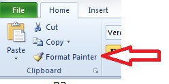 This is a fabulous little brush. Use it to copy the formatting from one cell to other cells. So if you had a group of cells that were formatted exactly as you wanted them, and you wanted to copy that formatting to another group of cells, all you do is highlight the formatted cells, click on the format painter, and then click on the cells you want to format. That's it.
Styles
The Styles Menu lets you easily format your cells to pre-designed formats. You can select from the options available by simply clicking on your preferred style type while you have your cell highlighted. You can also adjust the styles available, so for example make the text in the block "Accent 4" bold and italic, by right clicking on the "Accent 4" block and selecting "Modify".
These styles will apply to all your worksheets within a workbook. A nice way to ensure all your sheets look uniform and smart.
And now for something completely random....
I find this next tool really useful for highlighting specific cells. So, for example, you have filtered a number of rows, and you want to delete the data in your filtered cells, but leave the "hidden" rows untouched. You could delete each cell's data separately. You could trust in the goodness of Excel that if you just highlight all the cells and press delete it won't delete the underlying cells. (Sadly, this has happened to me once too often, and the trust has gone, so I am always extra cautious).
Or, you could just use the "Go To Special" tool, which you find here, right at the end of the home menu...
Click on this, and you get a table of various options you can select. For our example, you would use "Visible Cells only".
If you just wanted to select all the blank cells in a selection, you select (funnily enough) "Blanks" and so it goes on....
This is just a handy little tool for finding specific types of cells, and one that I have discovered not so many people are aware of.
So those are my random helpful icons for today. Again, if you have any questions, please feel free to add a comment or get in touch with this link.
Thanks for reading, and happy spreadsheeting!
Brand Beckham. Known worldwide. He is handsome but rugged, a man's kind of man on the field, a woman's kind of man with children and fashion. She is forever pouty, perfectly groomed, and her fashion label is growing beyond anyone's expectations...besides maybe her own.
So how do they do it? I'm no marketing guru, but what strikes me most about the couple is that there is almost a uniform look about them. Their looks never change too drastically, they have a style and they stick to it. Victoria's fashion lines are instantly identifiable as hers with their clean cut lines and simple, yet always smart, designs. I mean, who doesn't immediately recognise these two?
So well done them...branding done right. But do you know that you can brand your own Excel work? You can, I've done it. Most of my colleagues could open one of my workbooks and instantly say, "Oh Vicky, this is one of yours, isn't it?" How did I do it? I certainly didn't have "Vicky's workbook" emblazoned across the top. I try be a bit more subtle than that....
You may have noticed through my blogs that I like the colour blue. Well, most of my worksheets have dark blue headings, with white bold text. Any other lines that need highlighting underneath will be highlighted in lighter shades of blue. Borders will be done in blue. And there will be NO GRIDLINES!! (I hate gridlines, truly I do).
These simple things managed to somehow "brand" my workbooks so that they became easily identifiable as mine. Now, this may not seem important to you, but having workbooks always look the same will a) let your bosses know that the brilliant analysis floating around the company is yours, and b) make your spreadsheets easy to read.
You're probably thinking though that you couldn't be bothered re-doing all that formatting for all your new spreadsheets. The good news is, you don't have to. To have all your favourite settings lined up each time you open Excel is easy. Here is how:
Open a new, blank workbook and choose the way you would always prefer your workbooks to look by:
1) Selecting a theme. This decides the colours, fonts etc for your entire workbook. For more on this, read my earlier blog on formatting here.
2) Using your Styles toolkit. On your Home menu tab, you will find Styles midway across, with maybe 4 coloured boxes. Click on the downward arrow and you'll get a full choice like this:
Now, depending on the theme you have chosen, your Titles and Headings colours will be different.
If you prefer to always have any text in your workbook aligned to the middle of the cell and wrapped, or in Italics, or Bold, I would recommend making these changes to your "Normal" cell choice.
To adjust your "Normal" cell choice, just right click on the box, and select modify:
Click on the Format button that comes up, and adjust as you please. Click OK, and any cell in your workbook which is classified as Normal (which is all of them at this point), will be adjusted to your new settings.
You can adjust any of these cell types, so you could choose a heading type that you will always use, and make the font Bold. To then apply that formatting to your workbook, click on a cell you want to use as a heading, and click on that Heading button in the style box.
If you want to change it back to normal, click on the cell, and click on the Normal button again. (Note - you will need to change the alignment etc on your Heading buttons too).
3) Decide whether you want a header or footer on all your workbooks. If so, go to Insert - Text - Header & Footer. So for example, if you wanted the date and the file directory as a footer on each of your workbooks, click on Go to Footer in the Header & Footer toolbox, and you will get something that looks like this:
Click in the box where you want your footer to go (left, right or centre) and then click on your options above - so for our example you would click on Current Date and File Path.
Once you are done, click anywhere else on the sheet, and got to View - Normal to take your sheet out of the Page Layout mode.
4) Make any other changes you would like and make sure you are happy with the way your workbook now looks.
All these changes you have made now apply to the workbook you have open. To make all your new workbooks look like this, save your workbook as an Excel Workbook into your XLStart folder.
To find the address for this folder, go to File - Options - Trust Center - Trust Center Settings - Trusted Locations. The address will be the file path with XLStart in the file name. Click on the path, and the full address will appear below the box.
Once you have saved your workbook into that folder, everytime you open Excel, your new, branded Workbook will appear. And you can start spreading your own unique brand across the office!
A big thank you to the reader who sent in this week's request. Hope you found it useful. If you have specific query you would like covered, please leave a comment below.
If you would like to sign up to receive our weekly reminder of the blog, click here.
Happy spreadsheeting!


