So, we continue our "Back to Basics" blog run this week. I want to look at the "taken for granted and normally ignored" Home menu.
Yes, this menu contains so many tools that you probably use all the time, you would be forgiven for not investigating any of the more obscure icons. That is what I am for....
First off I want to go over some of my favourite tools for making your spreadsheets look good (and it's all about looking good, don't you know! ) I have gone over these in detail in a number of my previous blogs, but for a quick recap:
Format Painter
 This is a fabulous little brush. Use it to copy the formatting from one cell to other cells. So if you had a group of cells that were formatted exactly as you wanted them, and you wanted to copy that formatting to another group of cells, all you do is highlight the formatted cells, click on the format painter, and then click on the cells you want to format. That's it.
Styles
The Styles Menu lets you easily format your cells to pre-designed formats. You can select from the options available by simply clicking on your preferred style type while you have your cell highlighted. You can also adjust the styles available, so for example make the text in the block "Accent 4" bold and italic, by right clicking on the "Accent 4" block and selecting "Modify".
These styles will apply to all your worksheets within a workbook. A nice way to ensure all your sheets look uniform and smart.
And now for something completely random....
I find this next tool really useful for highlighting specific cells. So, for example, you have filtered a number of rows, and you want to delete the data in your filtered cells, but leave the "hidden" rows untouched. You could delete each cell's data separately. You could trust in the goodness of Excel that if you just highlight all the cells and press delete it won't delete the underlying cells. (Sadly, this has happened to me once too often, and the trust has gone, so I am always extra cautious).
Or, you could just use the "Go To Special" tool, which you find here, right at the end of the home menu...
Click on this, and you get a table of various options you can select. For our example, you would use "Visible Cells only".
If you just wanted to select all the blank cells in a selection, you select (funnily enough) "Blanks" and so it goes on....
This is just a handy little tool for finding specific types of cells, and one that I have discovered not so many people are aware of.
So those are my random helpful icons for today. Again, if you have any questions, please feel free to add a comment or get in touch with this link.
Thanks for reading, and happy spreadsheeting!
Well, pretty at least. When viewed on a spreadsheet. What am I on about, you may wonder. Bear with me...
Have you ever seen those photographs of celebrities where the poor girl has dared to leave the house without a bucket of makeup on? The horrors! The tabloids point out that she looks pretty normal without all the airbrushing and uplighting, and we all think, "We could walk right past her on the street and not notice".
The same goes for spreadsheets. They like a little lipstick and airbrushing. It makes them stand out. Don't believe me? Compare the two sets of exact same data below, showing the IRB top 8 rankings for the last 3 years, and the movements year on year:
Example A:
Example B:
Now, feel free to disagree with me, but I find example B easier to read (especially when its a 1000 lines of data over 30 columns you're analysing). You can immediately see who has moved up, who has moved down, and who has stayed consistently at the top (damn those Kiwis).
It took me all of about one and a half minutes to re-format the boring numbers in Example A to the clear and concise numbers in Example B. Here is how:
1) Lose the gridlines: See my earlier blog on how to do this...
2) Choose your theme (this only applies to Excel 2007 and 2010): A theme basically sets a colour chart and font for your workbook. It influences the colours you can pick for cells, graphs, pivot tables etc., so choose wisely. If you haven't done this before, here is how:
Go to Page Layout - Themes. The drop down arrow will show you all the theme choices with their basic colour range. Select your particular fancy, and you're set. Note that next to the 'Themes' box, you also have options to change only the colour, font or effects. Play away to your heart's content until you're happy.
Note that if you decide halfway through that you would prefer a different colour chart, change your theme. Everything will follow suit, but note your columns and rows may change size too, so check your print preview before printing.
Note, also, that you can skip this step. Your worksheet will show the standard Office colours.
3) Highlight your headings: Select cell B2, and using your menu options on your Home menu tab, change your background colour, text colour and make the text bold.
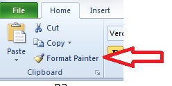
4) Use your format painter: For anyone who hasn't discovered this little gem, be prepared for a time saver of note. Go to your home menu tab and find this:
Point to it, right click, and add it to your your Quick Access toolbar, because you should be using this tool all the time. What this tiny little brush does is copy all your formatting in your highlighted cell and will apply this formatting to all other cells you select afterwards.
So you can use this to format all your headings in Row 4 in one go, by simply clicking on Cell B2, clicking on the format painter, and then selecting Cells B4:G4.
5) Center your data: by using the alignment buttons on your Home menu tab.
6) Center and merge: your main heading by selecting Cells B2:G2, then clicking the Merge & Center button in the alignment segment on the Home menu tab.
7) Use Conditional Formatting: to show the positives and negatives in the YOY columns. Select cells D5:D12. Still on the Home menu tab, drop down on the arrow on Conditional Formatting and select Highlight Cells - Greater than
Type in 0 in the box provided, and select your colour choice. I went for Green for anything that had a movement greater than 0. Then repeat for Less Than.
With your cells still selected, use the format painter to apply the same conditional formatting to cells F5:F12.
8) Apply borders: Note I left this till last. You really want to be happy that you have finished adding to your data before you apply borders, otherwise if you add anything later, you can spend a lot of wasted time redoing them.
I have chosen to add blue borders, as opposed to the standard black ones. To do this, select the cells you want a border around, and then go to
Home - Borders - More Borders.... Select your border style and colour FIRST, and then select where you want your border applied.
And you're done. The neat formatting might even distract you from the fact that Ireland has dropped four places in one year. Or not.
These are VERY simple formatting techniques. It can get a whole lot more complicated, but it very much depends on your data and what you will use it for.
For some helpful tips on other formatting techniques I have found handy over the years, sign up to our newsletter.
Happy Spreadsheeting!


